Recently I had conversations with several people on different occasions about effective goal setting. It is a common practice to use Specific, Measurable, Achievable, Relevant, and Time-bound (SMART) as criteria to create goals. However, using SMART goals for effective management or decision making is not as simple as it appears.
For example, “improve product ABC yield to 96% or more by September 30” can be a SMART goal. In a non-manufacturing environment, a similar goal can be “reduce invoices with errors to 4% or less by September 30.”
Suppose now is September 30, and we have only 4% of the products or invoices classified as bad. Did we achieve our goal?
Most people would say “Of course, we did.” But the real answer is “We don’t know without additional information or assumptions.”
Why?
The reason is that the 4% is calculated from a sample, or limited observations from the system or process we are evaluating. The true process capability may be higher or lower than 4%.
We can use a statistical approach to illustrate the phenomenon. Since the outcome of each item is binary (good/bad or with/without errors), we can model the process as a binomial distribution. Figure 1 shows the probability of observing 0 to 15 bad items if we examine a sample of 100 items, assuming that any item from the process has a 4% probability of being bad.
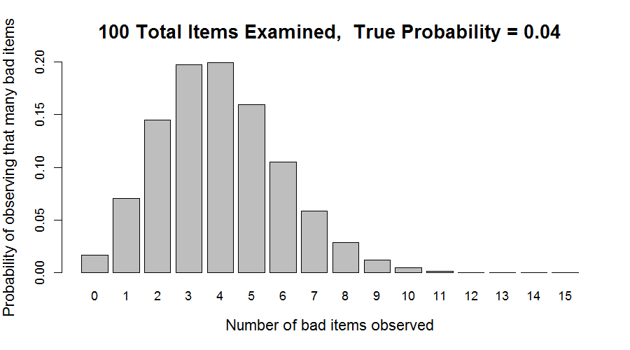
When the true probability is 4%, we expect to see 4 bad items per 100, on average. However, each sample of 100 items is different due to randomness, and we can get any number of bad items, 0, 1, 2, etc. If we add the probability values of the five leftmost bars (corresponding to 0, 1, 2, 3, and 4 bad items), the sum is close to 0.63. This means that there is only a 63% chance of seeing 4 or fewer bad items in a sample of 100, when we know the process should produce only 4% bad items.
More than 37% of the time, we will see 5 or more bad items in a sample of 100. In fact, there is a greater than 10% chance seeing eight bad items — twice as many as expected!
In contrast, a worse-performing process with a true probability of 5% (Figure 2) has a 44% chance of producing 4 or fewer bad items. This means that we will see it achieving the goal almost half the time.
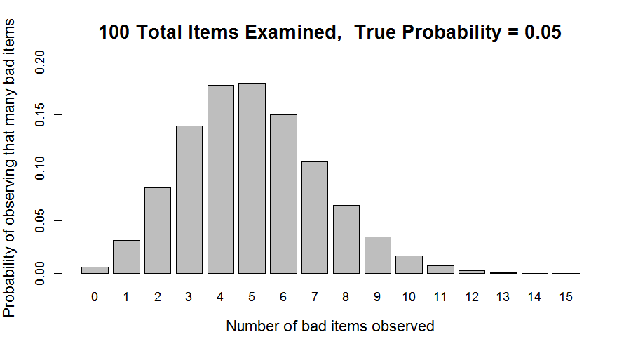
Suppose the first process represents your capability and the second one of your colleagues, how do you feel about using the SMART goal above as one criterion for raises or promotions?
The point I am making is not to abandon the SMART goals but to use them judiciously. In many cases, it calls for statistical thinking – understanding variation in data. Just because we can measure or quantify something doesn’t mean we are interpreting the data properly to make the right decision.
It takes “some rudimentary knowledge of science”1 to be smart.
1. Deming, W. Edwards. Out of the Crisis : Quality, Productivity, and Competitive Position. Cambridge, Mass.: Massachusetts Institute of Technology, Center for Advanced Engineering Study, 1986.
Comments
One response to “Setting SMART Goals”
[…] my blog Setting SMART Goals, I made the point that having a measurable goal in an improvement project is not enough — we […]